Evaluating Hockey Player Salaries through Regression Analysis in SPSS

- Question 1: Analyzing the Distribution of OTP in DEPOT_15 and DEPOT_18
- Solution
- Question 2: Analyzing the Relationship Between Player Characteristics and Earnings
- Solution
This comprehensive analysis showcases the application of the SPSS (Statistical Package for the Social Sciences) environment in a Regression Analysis assignment using SPSS to explore and draw meaningful conclusions from two distinct datasets. The study encompasses conducting regression analyses to evaluate the relationships between player attributes and earnings. The study tests multiple hypotheses, exploring the impact of factors such as birth quarter, age, height, weight, experience, captaincy, nationality, and position on player earnings.
Question 1: Analyzing the Distribution of OTP in DEPOT_15 and DEPOT_18
Problem Statement: You are tasked with examining the distribution of On-Time Performance (OTP) for two different depots, DEPOT_15 and DEPOT_18. Determine whether the OTP data for these depots follows a normal distribution and if an independent samples t-test is appropriate to compare them. This analysis aims to understand the characteristics of OTP data at these depots.
Solution
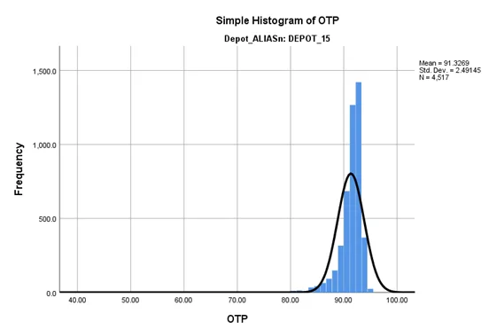
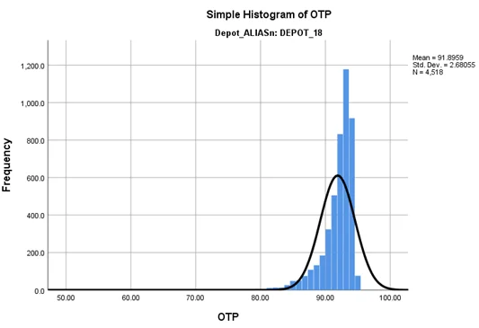
From the histogram of OTP for both DEPOT_15 and DEPOT_18, we can see that neither of them is normally distributed and are right skewed. Therefore, an independent samples t-test can’t be conducted on the OTP data.
Answer-2
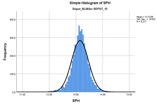
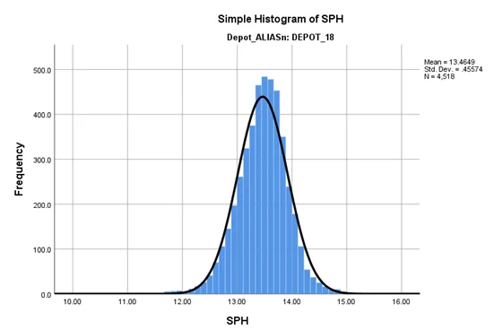
From the histogram of SPH for both DEPOT_15 and DEPOT_18, we can see that both of them are normally distributed. Therefore, an independent samples t-test can be conducted on the SPH data.
Group Statistics
| Depot_ALIASn | N | Mean | Std. Deviation | Std. Error Mean | |
|---|---|---|---|---|---|
| SPH | DEPOT_15 | 4517 | 13.1538 | .31831 | .00474 |
| DEPOT_18 | 4518 | 13.4649 | .45574 | .00678 |
Independent Samples Test
| Levene's Test for Equality of Variances | t-test for Equality of Means | |||||||||
|---|---|---|---|---|---|---|---|---|---|---|
| F | Sig. | t | df | Sig. (2-tailed) | Mean Difference | Std. Error Difference | 95% Confidence Interval of the Difference | |||
| Lower | Upper | |||||||||
| SPH | Equal variances assumed | 7.484 | .006 | -2.623 | 1006 | .009 | -.16938 | .06458 | -.29612 | -.04265 |
| Equal variances not assumed | -2.623 | 986.724 | .009 | -.16938 | .06458 | -.29612 | -.04265 | |||
In our independent sample t test, df=37.62 and p-value=0.000 since the p-value is less than 0.05 we can reject the null hypothesis and conclude that there is a statistically significant difference in SPH for the two depots.
Group Statistics
| Year | N | Mean | Std. Deviation | Std. Error Mean | |
|---|---|---|---|---|---|
| SPH | STOPS_PER_HR | 504 | 13.0559 | .95091 | .04236 |
| STOPS_PER_HR_2 | 504 | 13.2252 | 1.09456 | .04876 |
Independent Samples Test
| Levene's Test for Equality of Variances | t-test for Equality of Means | |||||||||
|---|---|---|---|---|---|---|---|---|---|---|
| F | Sig. | t | df | Sig. (2-tailed) | Mean Difference | Std. Error Difference | 95% Confidence Interval of the Difference | |||
| Lower | Upper | |||||||||
| SPH | Equal variances assumed | 7.484 | .006 | -2.623 | 1006 | .009 | -.16938 | .06458 | -.29612 | -.04265 |
| Equal variances not assumed | -2.623 | 986.724 | .009 | -.16938 | .06458 | -.29612 | -.04265 | |||
Since p-value for independent sample t-test is 0.009 which is less than 0.05 we can reject the null hypothesis and conclude that the intervention of swapping the Senior Managers between depots have a statistically significant impact on the stops per hour productivity at either depot.
Question 2: Analyzing the Relationship Between Player Characteristics and Earnings
Problem Statement: Explore the relationship between various player characteristics (birth quarter, age, height, weight, experience, captaincy, country of birth, and position) and player earnings. This analysis aims to assess the impact of these factors on player earnings and determine whether these relationships are statistically significant.
Solution
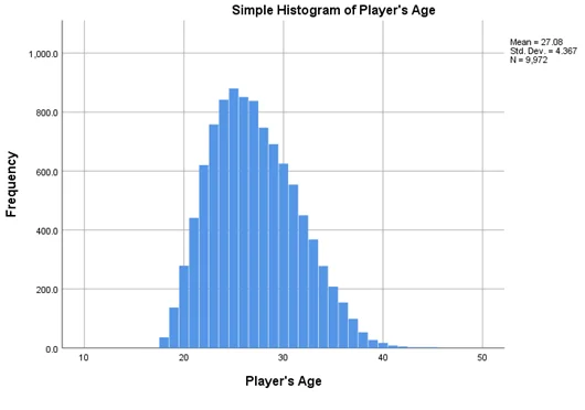
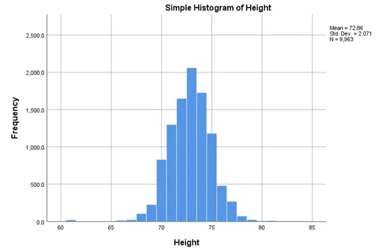
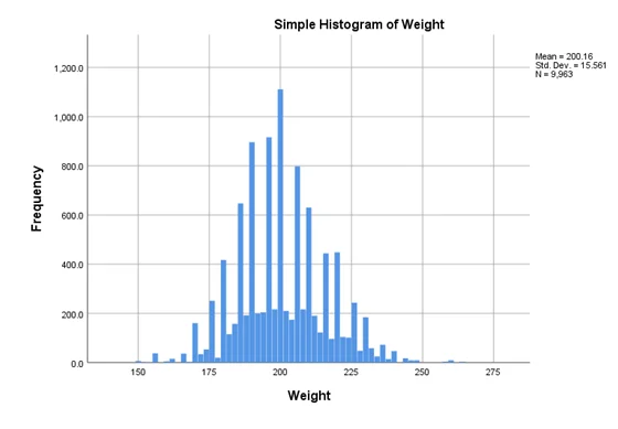
From the histograms we can see that these variables are approximately normally distributed. Therefore, all the assumptions for regression are met.
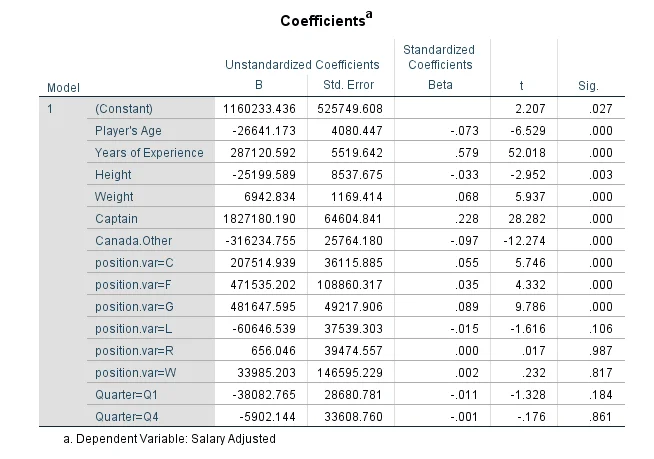
From the table of regression coefficients
Players born in the first quarter of the year (January, February and March) earn more than players born in the last quarter (October, November and December);
Answer- We can see that coefficient of Q1 is -38083 and Q3 is -5902 which is positive but they are not statistically significant. Therefore, we can’t say Players born in the first quarter of the year (January, February and March) earn more than players born in the last quarter (October, November and December).
Earnings have increased over the years covered by the data;
Answer-Yes
Earnings increase as players grow older;
Answer-We can see that coefficient of age is -26641.173 which is positive and is statistically significant (P-value=0.000). Therefore, we can say that Earnings decrease as players grow older
Earnings are positively related to a player’s height;
Answer- We can see that coefficient of player’s height is -25199.589 which is negative and it is statistically significant (P-value=0.003). Therefore, we can say that Earnings decrease as players height increase.
Earnings are positively related to a player’s weight;
Answer-We can see that coefficient of player’s weight is 6942.834 which is positive and it is statistically significant (P-value=0.000). Therefore, we can say that Earnings increase as players height increase.
Earnings are positively related to years of experience;
Answer- We can see that coefficient of experience is 287120.592 which is positive and it is statistically significant (P-value=0.000). Therefore, we can say that Earnings are positively related to years of experience
Captains earn more than players who are not captains;
Answer- We can see that coefficient of captain is 1827180.190 which is positive and it is statistically significant (P-value=0.000). Therefore, we can say that Captains earn more than players who are not captains
Canadian-born players earn more than players born in other all other countries
Answer- We can see that coefficient of player’s Canada. other is -316234.755 which is negative and it is statistically significant (P-value=0.000). Therefore, we can say that Canadian-born players earn less than players born in other all other countries.
In the same model, determine the position associated with the highest earnings
Answer- We can see that coefficient of player’s position corresponding to G(Goalie) and its value is 481647.595 and it is statistically significant (P-value=0.000). Therefore, the position associated with the highest earnings is Goalie.
You Might Also Like
Explore our diverse sample collection for insightful assignments covering fundamental concepts to advanced methodologies. Dive into a wealth of topics and solutions tailored to your needs. Unlock valuable knowledge and inspiration through our curated samples.
SPSS
SPSS
SPSS
SPSS
SPSS
SPSS
SPSS
SPSS
SPSS
SPSS
SPSS
SPSS
SPSS