- Question:
- DIRECTIONS
- Task 1:
- Task 2:
- Task 3:
- Solution:
- Task 1
- Residuals:
- Task 2
- Task 3
- R File
Welcome to our detailed sample solution for the linear regression assignment, crafted to showcase our linear regression assignment help. In this project, we delve into analyzing helminth infection data to explore its impact on cognitive and verbal abilities in children. By fitting a linear regression model in R, we demonstrate the practical application of regression techniques, from model fitting to the evaluation of assumptions. This example highlights our approach to handling real-world data and provides a clear illustration of how to interpret and validate linear regression results, ensuring you gain a solid understanding of the methodology and its application. For further guidance and personalized support, our team is here to provide expert help with statistics assignments.
Question:
DIRECTIONS
Soil Helminths and Development for scientific article
Helminth infections and cognitive/verbal ability in children – data: https://sldr.netlify.app/data/helminths.csv – code book (variable descriptions): https://sldr.netlify.app/data/helminthscodebook.csv
Get Started Work in a Quarto file;
you will download and submit the rendered PDF
You can read in and glimpse() your data with code like:
worms <- read.csv('https://sldr.netlify.app/data/helminths.csv') glimpse(worms)
Task 1:
Fit a model Return to the scientific article, if needed, to identify:
- What is a response variable that the authors used in a linear model in the paper?
- What predictor variables did they use to predict it?
You don’t have to replicate an analysis from the paper exactly; you can simplify a bit or modify if you wish. But if you can, plan something as close as possible to one of the “real” models. Use lm() to fit this model yourself in R, and show the model summary().
Task 2:
A Slope Look more carefully at one slope estimate from your model summary().
Does it seem to match what the authors found in the paper? If not, do you have an idea why not?
Task 3:
Assessment Check the L.I.N.E. conditions for your fitted model. For each one, show the needed graph; then, note which condition you are checking, whether you think it is met, and what evidence you see in the graph to support your choice. Remember, if ANY of the conditions are not met, then the model is not to be trusted at all! If you find an unmet condition, do you think this means there could be a problem with the published paper, or no? R code is provided that should be useful in the process. (Of course, you will need to change model and dataset to whatever name you use for your fitted model and your dataset.)

Solution:
Task 1
The response variable utilized in the linear model within the paper pertains to the cognitive score of preschool children. This cognitive score serves as a quantitative measure reflecting the cognitive development and functioning of the children under study.
In contrast, the predictor variables encompass a range of factors presumed to potentially impact cognitive development in preschool children. These factors include the cumulative infection statuses of Ascaris, Trichuris, and any soil-transmitted helminth (STH), highlighting the potential influence of parasitic infections on cognitive outcomes. Furthermore, the predictor variables include socio-economic indicators such as the mother's education level, operationalized as the completion of secondary school, and household characteristics such as the cooking method and toilet facilities. Stunting at one year, an indicator of malnutrition and growth impairment, is also included as a predictor variable. Additionally, the Bayley-III cognitive raw score at one year is integrated as a predictor, capturing cognitive functioning at an earlier developmental stage. Other variables incorporated into the model encompass the number of healthy growth visits attended from birth to one year of age and the age of the child at the time of assessment. These predictor variables collectively represent a broad spectrum of influences potentially shaping cognitive development in preschool-aged children, encompassing both biological and socio-environmental determinants.
lm(formula = cog_composite ~ AscKKD12 + TrichKKD12 + AnyKKD12 +
Mated_sec + Cocinar_gas + Bano_tasa + stunting1 + cog_raw3 +
CRED_12 + age24, data = worms)
Residuals:
| Min | 1Q | Median | 3Q | Max |
|---|---|---|---|---|
| -28.7225 | -6.3337 | 0.3253 | 6.0713 | 28.2844 |
| Coefficients | Estimate | Std. Error | t value | Pr(>|t|) |
|---|---|---|---|---|
| Intercept | 120.822 | 11.2254 | 10.763 | < 2e-16 |
| AscKKD12 | -0.9373 | 3.51208 | -0.267 | 0.78964 |
| TrichKKD12 | 2.25044 | 2.70028 | 0.833 | 0.40484 |
| AnyKKD12 | 1.27719 | 3.59948 | 0.355 | 0.72281 |
| Mated_sec | 1.0776 | 0.72624 | 1.484 | 0.13823 |
| Cocinar_gas | 0.23247 | 0.73973 | 0.314 | 0.75339 |
| Bano_tasa | 2.55103 | 0.69238 | 3.684 | 0.00024 |
| stunting1 | -2.5063 | 0.76504 | -3.276 | 0.00109 |
| cog_raw3 | 0.35208 | 0.10028 | 3.511 | 0.00047 |
| CRED_12 | 0.05323 | 0.09313 | 0.572 | 0.5678 |
| age24 | -18.359 | 4.98527 | -3.683 | 0.00025 |
Residual standard error: 9.343 on 865 degrees of freedom
(4 observations deleted due to missingness)
Multiple R-squared: 0.07767, Adjusted R-squared: 0.067
F-statistic: 7.284 on 10 and 865 DF, p-value: 3.959e-11
Task 2
In our model, the estimated coefficient for AscKKD12 is -0.93726, suggesting that, on average, the cognitive composite score decreases by approximately 0.94 points for each unit increase in the cumulative Ascaris infection status.
Comparing this with the findings reported in the paper, the univariable and multivariable beta coefficients for Ascaris infection status range from approximately -0.64 to -1.98. These values are somewhat similar to the coefficient estimate obtained in our model. Therefore, for the predictor variable `AscKKD12`, the estimated effect size in our model seems to be consistent with the effect sizes reported in the paper, indicating a negative association between cumulative Ascaris infection status and cognitive scores in preschool children.
Task 3
To check the L.I.N.E. conditions for the fitted model, we need to examine:
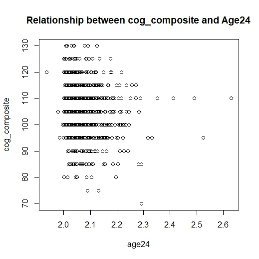
Linearity: This condition requires that the relationship between the predictor variables and the response variable is linear. We can check this condition by plotting the observed values of the response variable against the predicted values from the model.

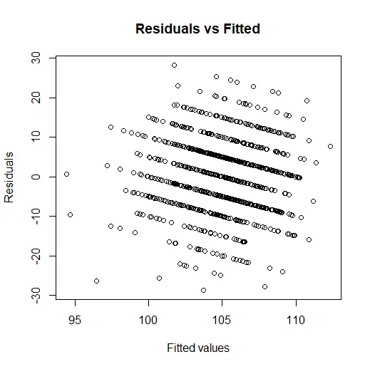
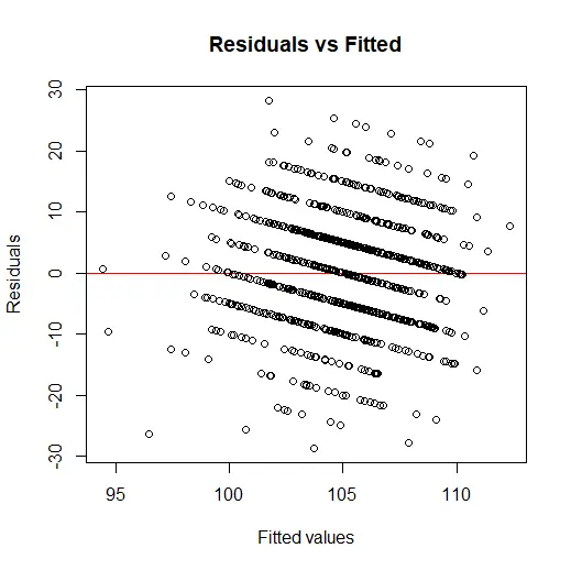
Independence: This condition requires that the residuals (the differences between observed and predicted values) are independent of each other. We can check this condition by plotting the residuals against the predicted values.

Normality: This condition requires that the residuals are normally distributed. We can check this condition by plotting a histogram of the residuals or a Q-Q plot comparing the residuals to a normal distribution.

Equal Variance: This condition, also known as homoscedasticity, requires that the variability of the residuals is constant across all levels of the predictor variables. We can check this condition by plotting the residuals against the predicted values or against each predictor variable.

R File
worms <- read.csv("helminths.csv",sep=",")
attach(worms)
model <- lm(cog_composite ~ AscKKD12 + TrichKKD12 + AnyKKD12 + Mated_sec + Cocinar_gas + Bano_tasa + stunting1 + cog_raw3 + CRED_12 + age24, data = worms)
summary(model)

# Load the dplyr package
library(dplyr)
dataset<-worms|>mutate(resids=resid(model),model_values=predict(model))

# Filter out missing values before applying the model
worms_filtered <- na.omit(worms)

# Apply mutate function
dataset <- worms_filtered|> mutate(resids = residuals(model), model_values = predict(model))

#scatter plot of data
gf_point(cog_composite ~ AscKKD12,data=worms)

#residuals vs fitted
gf_point(resids~model_values, data=worms)

#histogram of residual
gf_histogram(~resids, data=worms)

#ACF plot
s245::gf_acf(~model)
Similar Samples
We provide high-quality statistics assignment services tailored to students' needs. Browse through our sample questions to assess the quality of our work. Trust us for timely, accurate solutions that simplify complex statistical problems, helping you achieve academic success effortlessly.
Statistics
STATA
Statistics
SPSS
Data Analysis
Statistics
SPSS
Statistics
Statistics
Statistics
Statistics
Statistics
Statistics
Statistics
Statistics
Statistics
Statistics
Statistics
Statistics
Statistics
