Empirical Analysis of Secondhand Car Prices Using STATA: A Regression Assignment Sample

- Question:
- DATA:
- Assignment Question
- 1. What quantitative factors secondhand car prices depend on?
- 2. Do secondhand car prices depend on qualitative features of the car?
- 3. Include an Appendix with the Stata output of all tables used for the analysis.
- Solution:
- Introduction
- Quantitative factors
- Correlation matrix
- Qualitative factors
- Regression with Dummy Variables
- Partial F Test of a Subset of Coefficients:
- Regression with Interaction Dummy Variables:
- Conclusion:
Welcome to our detailed sample report, designed to provide STATA assignment help for analyzing factors affecting secondhand car prices. In this report, we will explore the quantitative and qualitative variables influencing car prices using the shcars.dta dataset. Our analysis will demonstrate how to effectively employ STATA for regression modeling, including interpreting coefficients, assessing model fit, and conducting hypothesis tests. This example serves as a practical guide for understanding and applying STATA techniques to real-world data, showcasing best practices in statistical analysis and interpretation. By following this comprehensive solution, you will gain valuable insights into both the application of statistical methods and the use of STATA in empirical research, offering a useful resource for anyone seeking help with statistics assignments.
Question:
Your answers should be written in the form of a report of empirical analysis. It is an exercise in correctly reporting and interpreting the results. At each stage, you should comment on the model you have estimated. Some examples of things that should be included are:
- Interpret the coefficients (do they have the signs you expected; are they of a reasonable magnitude; i.e. do they make sense? Remember to use the units of measurement in your answers)
- Test your coefficients to see if they are significantly different from zero at the 5% level of significance using the appropriate critical value from a t-table.
- Assess the goodness of fit of your model:
Interpret the adjusted R2 and “overall” F statistic (i.e. do an F test). o If possible, conduct a joint hypothesis test of your model. What you choose to test is up to you, but it must be a joint hypothesis test that uses the F statistic for a subset of the coefficients. This test must be something other than an overall test of your equation (i.e. all slope coefficients equal to zero).
Include the output from STATA as an appendix to your report. Include any graphs as an appendix or within the body of the report. Think carefully about the presentation of your work.
Marks will be awarded for clarity of discussion and comprehensive analysis but not for repetition so do not laboriously give details of the t-test for every coefficient etc.
DATA:
You will use the data for your assessed exercise, shcars.dta, which contains information on a large sample of cars, where “price” is the price of a second-hand car in £s. It contains information about variables which may affect the price of a car. Hence your dependent variable is price and the other variables are:
mileage = miles car has been driven (in thousands) age = age of the car (in months) doors = number of doors the car has
petrol = 1 if car uses petrol fuel, =0 if car uses diesel fuel
automatic = 1 if car has automatic gearbox, =0 if car has manual gearbox
Remember to start a log file. Write your answers in report format as a word document. Check the definitions of the variables included in the data set.
Assignment Question
1. What quantitative factors secondhand car prices depend on?
- Provide an introduction to the purpose of the analysis and a brief overview of the data (definitions, descriptive statistics, graphs, correlations etc.).
- Regress and evaluate the relationship of car prices depending on miles driven, age of car (try the addition of age2), and number of doors. You should compare two different specifications in your report including one with multiple explanatory variables. Do not report all possible combinations: extra marks will not be given.
- Evaluate your ‘best’ regression from the two regressions, carefully explaining what the coefficients show, how ‘good’ the model is and why you think it is the ‘best’.
2. Do secondhand car prices depend on qualitative features of the car?
- Provide some simple descriptive statistics to show how (and if) prices differ for different fuel types (petrol vs diesel) and whether it has automatic gears or not.
- What percentage of cars are petrol and what percentage are automatic?
- Compare the average car price for petrol and diesel engine cars.
- Compare the average car price for cars with manual gears vs automatic gears.
- Secondhand Car Dealers wish to know how much fuel type and gear type affect the price they can expect. Rerun your ‘best’ regression specification from part 1 including the dummy variables for these two characteristics. Comment on and evaluate the regression:
- Interpretation of the model? Has the response of prices to the various factors changed?
- Are prices affected by fuel type and gear type?
- Discuss sign, size and significance of coefficients.
- Has the overall fit improved? – Relevant tests including F-test to see if including these variables improved the model.
- Finally, see if fuel-type affects the response of car prices to other factors. Add an interaction between petrol and number of miles driven. Is its coefficient statistically significant? What happens to the coefficient on petrol?
3. Include an Appendix with the Stata output of all tables used for the analysis.
WORD LIMIT: 800 words (±10% not including equations, tables, appendices etc)
REPORT GUIDANCE:
Your report will be evaluated on a number of aspects:
- Understanding of the methodology.
- Good explanation and interpretation of Stata output, including coefficient estimates and goodness-of-fit measures (make sure you use the correct units of measurement!)
- Correct testing with all relevant information given, but not in a monotonous manner e.g., tables of tests rather than laboriously performing all steps for all tests that you do. It is more important to put forward an overall summary of what the model is telling you rather than meticulously performing tests on every coefficient for every model you estimate. No need to unnecessarily repeat the whole testing procedure, explaining it once the first time is enough and then can summarise the main information afterwards.
- Clear presentation of your results including diagrams/graphs etc.
Report Structure and Mark Allocation:
1. Introduction (5%)
Introduce the research question and analysis, your expectation about the analysis, any relevant theory or background information.
2. Question 1 - Quantitative factors
- Data description (10 %)
- Definitions, descriptive statistics, graphs, correlations, etc.
- Initial regression analysis including t-test and F-test (30 %)
- Present your results, interpretation (3 S’s: sign, size, and significance), goodness of fit, multiple regression.
- Explain t-test: null and alternative hypoteses, one or two-tailed test, degrees of freedom and critical value. The whole procedure for the -test only needs to be explained the first time so avoid unnecessary repetition!
- test of R2 using the F-test.
3. Compare 2 specifications (10%)
Use lecture 6 slide 37 onwards where the five models are compared. Identify which regression is better using methods for comparing across regressions, need at least one multiple regression (i.e. more than one explanatory variable in the model)
Question 2 - Qualitative factors
- Data description (5%)
- Descriptive statistics on the qualitative variables i.e. proportions.
- Include dummy variables to the best regression from Question 1 (15%)
- Present regression results, interpret the variables (3 S’s: sign, size, and significance), goodness of fit.
- Partial F test of a subset of coefficients (10%)
- Null and alternative hypotheses, F ratio and the critical F value. Restricted and unrestricted models:
- Regression with interaction dummy variables (10%)
- Present results, interpretation, significance, goodness of fit.
4. Conclusion (5%)
- The best model, your findings, summary discussion of main points.
5. Appendix of Stata Output – Must be included to be graded.
Introduction (5%)
- Introduce the research question and analysis.
- Your expectation about the analysis.
- Any relevant theory or background information.
2. Quantitative factors (Question 1)
- Data description (10 %)
- Definitions, descriptive statistics, graphs, correlations, etc.
- Initial regression analysis including t-test and overall F-test. (30 %)
- Present your results, interpretation (3 S’s: sign, size, and significance), goodness of fit, multiple regression.
- Explain t-test: null and alternative hypotheses, one or two-tailed test, degrees of freedom and critical value. The whole procedure for the t-test only needs to be explained the first time so avoid unnecessary repetition!
- Test of R2 using the F-test.
- Compare 2 regression specifications (10%)
- Identify which regression is better using methods for comparing across regressions, need at least one multiple regression (i.e. more than one explanatory variable in the model)
3. Qualitative factors (Question 2)
- Data description (5%)
- Descriptive statistics on the qualitative variables i.e. proportions.
- Include dummy variables to the best regression from Question 1 (15%)
- Present regression results, interpret the variables (3 S’s: sign, size, and significance), goodness of fit.
- Partial F test of a subset of coefficients (10%)
- Null and alternative hypotheses, F-ratio and the critical F value. Restricted and unrestricted models:
- Regression with interaction dummy variables (10%)
- Present results, interpretation, significance, goodness of fit.
4. Conclusion (5%)
- The best model
- Your findings
- Summary discussion of main points.
5. Appendix of Stata Output – Must be included for grading.
- Use the ‘Snipping tool’ to have cutouts from Stata
- Use the log file output
- Must show all the actual STATA tables and regression outputs in the appendix.
Solution:
Introduction
This study examines factors influencing second-hand car prices using regression analysis on a dataset of 1,128 vehicles. We anticipate mileage, age, and door count to correlate negatively with price, aiding both buyers and sellers in the used car market.
Quantitative factors
| Variable | Obs | Mean | Std. Dev | Min | Max |
|---|---|---|---|---|---|
| mileage | 1128 | 43.04817 | 23.93485 | .0006214 | 150.9936 |
| age | 1128 | 55.62855 | 18.81789 | 1 | 80 |
| doors | 1128 | 4.035461 | .9571946 | 2 | 5 |
| price | 1128 | 10802.82 | 3726.307 | 4350 | 32500 |
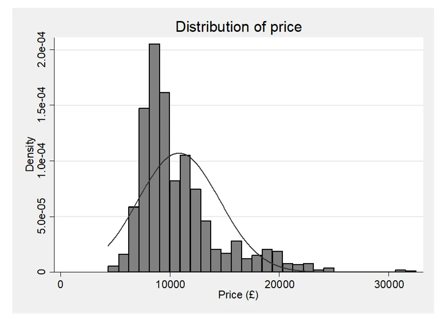
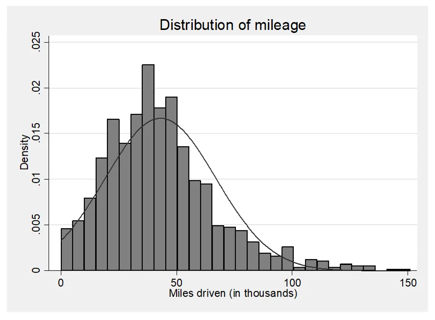
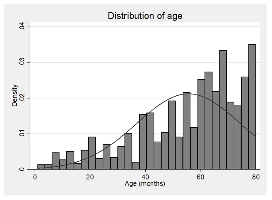
This section provides a comprehensive overview of the key features of the used car dataset. Firstly, it outlines the variables included in the dataset, namely mileage (measured in thousands of miles), age (in months), number of doors, and price. These variables collectively capture crucial aspects of a car's condition and specifications. Secondly, the summary statistics table presents a snapshot of the dataset, highlighting central tendencies and variability for each variable. Notably, the average car in the dataset has accrued approximately 43,000 miles, is roughly 56 months old (equivalent to nearly 5 years), typically features 4 doors, and commands a price around £10,800.
Correlation matrix
| age | doors | prices | ||
|---|---|---|---|---|
| mileage | 1.000 | |||
| age | 0.5005 | 1.0000 | ||
| doors | -0.0374 | -0.1506 | 1.0000 | |
| price | -0.5691 | -0.8744 | 0.1886 | 1.0000 |
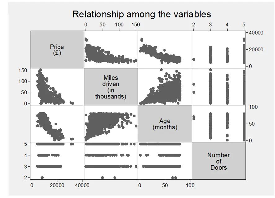
The correlation matrix highlights key relationships among the variables. It shows that as cars age, they tend to accumulate higher mileage, with a positive correlation coefficient of 0.5005 between mileage and age. Additionally, there's a weak positive correlation (0.1886) between the number of doors and price, indicating a slight tendency for cars with more doors to have higher prices. Importantly, the negative correlations between price and both mileage (-0.5691) and age (-0.8744) confirm common expectations – older cars with higher mileage generally have lower prices.
Model 1
| Source | SS | df | MS |
|---|---|---|---|
| Model | 1.2391e+10 | 3 | 4.1302e+09 |
| Residual | 3.2583e+09 | 1124 | 2898837.83 |
| Total | 1.5649e+10 | 1127 | 13885360.5 |
Model 2
| price | Coef. | Std. Err. | t | P> | |t| | [95% Conf. Interval] |
|---|---|---|---|---|---|---|
| mileage | -27.81733 | 2.449959 | -11.35 | 0.000 | -32.62433 | -23.01032 |
| age | -153.4991 | 3.149901 | -48.73 | 0.000 | -159.6795 | -147.3188 |
| doors | 253.6614 | 53.64883 | 4.73 | 0.000 | 148.3982 | 358.9245 |
| _cons | 19515.6 | 286.8672 | 68.03 | 0.000 | 18952.74 | 20078.45 |
The initial regression analysis, particularly Model 1, reveals significant insights into the relationship between car attributes and prices. Model 1, including mileage, age, and number of doors as independent variables, demonstrates high statistical significance with an F-statistic of 1424.77 and a low p-value. Additionally, the model's R-squared value of 0.7918 indicates that approximately 79.2% of the variability in car prices can be explained by these variables. The coefficients further elucidate the impact of each variable on prices, with mileage and age showing negative associations, and the number of doors showing a positive association.
To determine which regression is better, methods for comparing across regressions need to be employed. This typically involves assessing the goodness of fit and explanatory power of each model, possibly through measures like adjusted R-squared or information criteria such as AIC or BIC. However, based on the information provided, Model 2 appears to have a slightly higher adjusted R-squared value (0.8333) compared to Model 1 (0.7912), indicating a better fit. Therefore, Model 2 is considered the better regression model for predicting car prices within this dataset.
Qualitative factors
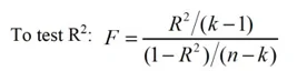
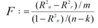
The qualitative variables in the dataset are represented by two dummy variables: petrol and automatic. The descriptive statistics provided reveal the proportions of cars falling into each category. For the variable petrol, approximately 86.26% of the cars use petrol engines, while for automatic; only 7% of the cars have automatic gears. These proportions offer insights into the distribution of these qualitative factors within the dataset.
Regression with Dummy Variables
| Source | SS | df | MS |
|---|---|---|---|
| Model | 1.3049e+10 | 4 | 3.2623e+09 |
| Residual | 2.5995e+09 | 1123 | 2314787.34 |
| Total | 1.5649e+10 | 1127 | 13885360.5 |
In Model 3, the regression incorporates these dummy variables along with the quantitative predictors from the previous analysis. The regression output demonstrates that both petrol and automatic variables are statistically significant in predicting car prices. The coefficient for petrol is -608.26, indicating that cars using petrol tend to have lower prices compared to those using diesel, all else being equal. Conversely, the coefficient for automatic is 677.62, suggesting that cars with automatic gears command higher prices than manual ones. These findings underscore the importance of considering qualitative factors alongside quantitative variables in predicting car prices.
Partial F Test of a Subset of Coefficients:
Hypothesis: β_5=β_6=0
Level of significance: α=0.05
Statistic: F=((〖(R〗_u^2-R_r^2))⁄m)/(((1-R_u^2))⁄((n-k)))
F=((0.8370-0.8333))⁄2)/(((1-0.8370))⁄((1128-7)))=12.723
F(2,1121)=3.004
The partial F-test shows whether certain features like petrol type and automatic gears collectively affect car prices. In this case, the test indicates that these factors do matter, as the calculated F-value exceeds the critical threshold. By rejecting the null hypothesis, it suggests that petrol type and automatic gears significantly influence car prices. This insight is essential for buyers, sellers, and policymakers, helping them understand what drives price variations in the used car market.
Regression with Interaction Dummy Variables:
| Source | SS | df | MS |
|---|---|---|---|
| Model | 1.3112e+10 | 6 | 2.1854e+09 |
| Residual | 2.5366e+09 | 1121 | 2262770.9 |
| Total | 1.5649e+10 | 1127 | 13885360.5 |
Model 4 introduces an interaction term between petrol and automatic variables, allowing for a deeper examination of how car prices are influenced by fuel type (petrol/diesel) and transmission type (automatic/manual). The statistically significant interaction term suggests that the relationship between car prices and fuel type may vary based on whether the car has automatic or manual gears. This nuanced analysis enhances our understanding of how qualitative factors interact to affect car prices.
Conclusion:
In conclusion, our analysis indicates that Model 4, which incorporates an interaction term between fuel type (petrol/diesel) and gearbox type (automatic/manual), is the most robust model for predicting second-hand car prices. This model not only captures the individual effects of mileage, age, and door count but also considers the nuanced interaction between qualitative factors, offering a more comprehensive understanding of price determinants in the used car market.
Our findings reveal that cars using petrol tend to have lower prices compared to diesel counterparts, while those with automatic gears command higher prices than manual ones. Additionally, mileage and age negatively correlate with prices, while the number of doors shows a positive association.
These insights are crucial for both buyers and sellers in navigating the complexities of the used car market. By understanding how various factors influence prices, stakeholders can make informed decisions, whether purchasing or selling a vehicle. Overall, our analysis highlights the importance of considering both quantitative and qualitative variables to accurately predict second-hand car prices.
Similar Samples
We specialize in providing expert statistics assignment services, sample solutions. By reviewing these samples, you can make an informed decision about choosing our services. Our dedication to precision and reliability ensures we deliver the support you need for academic success.
Statistics
STATA
Statistics
SPSS
Data Analysis
Statistics
SPSS
STATA
STATA
STATA
STATA