Implementing the EM Algorithm for Gaussian Mixture Models in Multivariate Statistics

- Question:
- Solution:
- EM-algorithm with gaussian mixture model
- Results
Welcome to our comprehensive sample solution for the multivariate statistics assignment, designed to provide multivariate statistics assignment help. In this example, we illustrate the practical application of advanced statistical techniques, focusing on the implementation of the Expectation-Maximization (EM) algorithm for Gaussian mixture models. This assignment covers key concepts such as parameter estimation, hypothesis testing, and iterative optimization, providing a detailed step-by-step guide to understanding and applying the EM algorithm in multivariate statistics. If you're looking for help with statistics assignments, this example will serve as a valuable resource for mastering complex topics. Through this example, you will learn how to approach complex statistical problems and enhance your proficiency in statistical modeling and analysis.
Question:
Solution:
EM-algorithm with gaussian mixture model
The observations are the visible variables in a Gaussian mixture model; the means, variances, and weights of the mixture components are the latent variables, which are the assignments of data points to mixture components.
The probability of the visible variables given the parameters is p(y|θ) that we call the likelihood. The EM algorithm seeks to identify the parameters θ that maximize the likelihood. Iteratively, the EM algorithm converges to a local maximum.
To represent an arbitrary distribution of the latent variables, z, we will use the notation q(z).
Mathematical transformations and operations allow us to write the following equation:
log p(y│θ) = ∫_ ^ ▒q(z) log (p(y│z, θ)p(z│θ))/q(z) dz + ∫_ ^ ▒q(z) log q(z)/(p(z│y, θ) ) dz
The term ∫_ ^ ▒q(z) log q(z)/(p(z│y,θ) ) dz = KL[q(z), p(z│y,θ)] is non-negative. Therefore, we obtain a lower bound for the logarithmic marginal likelihood:
L(q,θ)=∫_ ^ ▒q(z) log (p(y│z,θ)p(z│θ))/q(z) dz
The key idea behind the EM-algorithm is to maximize the lower bound L(q,θ) w.r.t q and parameters θ . However, we need q to estimate θ and we need θ to estimate q . Therefore, the EM-algorithm works iteratively in 2 steps: Expectation step and Maximization step:
- We initialize parameters θ = θ^(n=0)
- For each iteration over n:
- E step: we fix θ = θ^(n-1), and we maximize the lower bound L(q,θ) w.r.t q . If we recall the first equation, we have logp (y│θ) = L(q,θ) + KL[q(z), p(z│y,θ)]. Since logp (y│θ) is independent of q , maximizing L(q,θ) is equivalent to minimizing KL[q(z), p(z│y,θ)]. Therefore, the optimal value of q is q^(n*)=p(z│y,θ^(n-1) ).
- M step: we fix q to the value from the previous step q^(n*) and we maximize the lower bound L(q,θ) w.r.t. θ .
- We keep iteration until the difference between 2 consecutive values of the lower bound is less or equal than a defined threshold.
- Once the threshold reached, we achieve convergence of the EM-algorithm and we retrieve the optimal values of q and θ .
In this assignment, we will apply the EM-algorithm to estimate the parameters of gaussian mixtures with two gaussian sources. We consider 3 random variables as follows:
- I distributed Ber(p), with p ∈ [0.25,0.5]
- N_0 the Gaussian random variable N(μ_0,σ_0^2 ), with μ_0 ∈ [0,2] and σ_0 ∈ [2,4]
- N_1 the Gaussian random variable N(μ_1,σ_1^2 ), with μ_1 ∈ [4,6] and σ_1 ∈ [2,6]
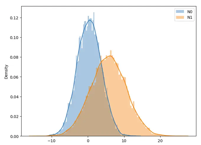
Plot of two gaussian random variables with random parameters
The algorithm is written in the following structure:
- Choice of random parameters: initial parameters are initialized wrt to the assignment.
- Data generation: data is generated per the random variable I , where each data point i is distributed according to N_(I_i ) (N_0 or N_1).
- E step: this step relies on calculating the matrix of responsibilities. Each row of the matrix represents a sample (data point) and each column represents a class (which means a gaussian source in our case, since we have two gaussian sources and therefore 2 classes). Thus, a responsibility represents the probability that the corresponding sample belongs to the corresponding class with the given (old) parameters: responsibility_z^i = p(Z=z│X=x_i,θ^k ). We then normalize the matrix to ensure having valid probabilities.
- M step: we maximize our function given the responsibilities and calculate the new parameters. We then update the values of means, stds and classes probabilities.
- Likelihood threshold: we calculate the log likelihood wrt to the new parameters and substract the old value of log likelihood stored in the previous iteration. If the threshold (0.001) isn’t reached, the algorithm continues iterating until this condition is met.
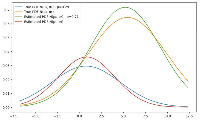
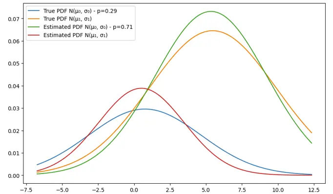
- Plot results: when the algorithm finishes, we plot PDFs with true and estimated parameters.
Results
We run 5 examples with different number of iterations. We will show in this document the plots. The prints are included in the notebook and easy to read.
Example 1: N_samples=100, n_iterations = 3
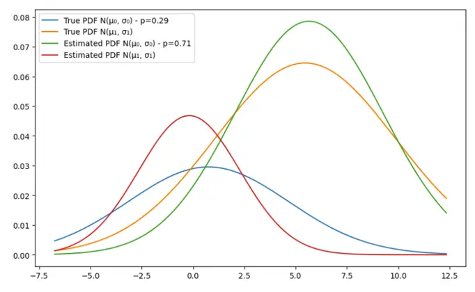
Example 2: N_samples=100, n_iterations = 5
Example 3: N_samples=100, n_iterations = 10
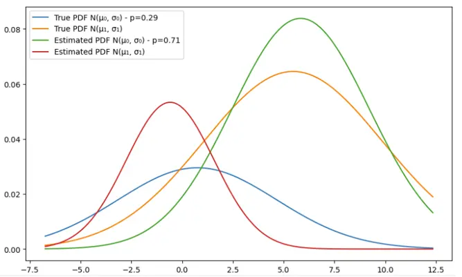
Example 4: N_samples=100, n_iterations = 100
| Parameters | Experiences | 1 | 2 | 3 | 4 |
|---|---|---|---|---|---|
| μ_0 | True | 0.78 | 0.75 | 0.75 | 0.75 |
| Estimate | 0.81 | 0.51 | -0.18 | -0.59 | |
| σ_0^2 | True | 3.90 | 3.90 | 3.90 | 3.90 |
| Estimate | 3.19 | 2.96 | 2.46 | 2.16 | |
| μ_1 | True | 5.46 | 5.46 | 5.46 | 5.46 |
| Estimate | 5.22 | 5.34 | 5.65 | 5.83 | |
| p | True | 4.39 | 4.39 | 4.39 | 4.39 |
| Estimate | 3.95 | 3.88 | 3.61 | 3.38 | |
| σ_1^2 | True | 0.29 | 0.29 | 0.29 | 0.29 |
| Estimate | 0.29 | 0.29 | 0.29 | 0.29 |
We can notice that for the second gaussian, the parameters are fairly close and the estimation is approximately giving close estimations. The mean however of the first guassian is declinig from the true value and the more the number of iterations increases, the bigger the gap between the true and estimated means. That can be explained by the low number of samples (100). Let’s double this number in the next example.
Example 5: N_samples=200, n_iterations = 3
Here, we can see almost a perfect estimation of the parameters for a low number of iterations, which can be explained by the number of samples that allows the algorithm to have enough data points to return a good estimation.
Similar Samples
We offer expertly solved Statistics assignment samples for students to explore. By reviewing these samples, you can assess the quality of our work and make an informed decision about using our services. We are committed to delivering precise and reliable assistance to ensure your academic success.
Statistics
STATA
Statistics
SPSS
Data Analysis
Statistics
SPSS
Statistics
Statistics
Statistics
Statistics
Statistics
Statistics
Statistics
Statistics
Statistics
Statistics
Statistics
Statistics
Statistics