Exploring Well-Being Factors with Statistics on BMI, Blood Pressure, and Age Using R Programming
- Problem Description
- Part 1: Investigating BMI Across Time in Australia
- Part 2: Examining the Relationship between Age and Systolic Blood Pressure
- Part 3: Exploring Correlations Between Time in Australia and Hypertension
Problem Description
In the R Programming assignment, we delve into a dataset containing 60 observations and 6 variables gathered from the LWM-LMP program. Among these variables are three continuous ones: BMI, Systolic blood pressure, and Age, as well as three categorical variables: time spent in Australia, socioeconomic status, and the presence of hypertension. Our analysis will primarily emphasize the application of statistical techniques and the utilization of R programming to address key research questions.
Part 1: Investigating BMI Across Time in Australia
Research Question: Is there a significant difference in the mean BMI among participants who spent varying durations in Australia, classified into five categories: >20 years, 1-5 years, 6-10 years, 11-20 years, and less than 12 months?
Analysis
We initiated our analysis with the calculation of descriptive statistics for BMI across the different time categories. The boxplot and a table of these statistics are presented below.
| Variable | Time | Mean | Std. Dev | Variance | Range |
|---|---|---|---|---|---|
| BMI | 20 years | 28.28 | 6.69 | 44.73 | 23.80 |
| 1-5 years | 24.85 | 4.33 | 18.77 | 14.52 | |
| 11-20 years | 32.14 | 7.83 | 61.38 | 23.30 | |
| 6-10 years | 29.63 | 4.46 | 19.89 | 14.10 | |
| 12 months | 27.38 | 5.96 | 35.54 | 21.99 |
Table 1: Descriptive Statistics for BMI by Time
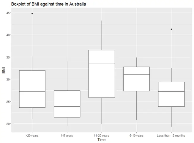
Figure 1: Boxplot of BMI against Time
After observing the descriptive statistics and the boxplot, we noticed that there is no significant difference in BMI across different durations of time spent in Australia. However, two outlier points were identified - one in the '>20 years' category and another in the '<12 months' category.
Given these observations, we conducted an ANOVA test to assess whether there is a statistically significant difference in the average BMI across the different time categories. The null and alternative hypotheses were defined as follows:
- H0: μ1 = μ2 = μ3 = μ4 = μ5 (No significant difference)
- H1: At least one mean is different
The significance level was set at 5%. The ANOVA results are summarized in the table below.
| Source of Variation | DF | Sum Sq | Mean SQ | F-Value | P-value |
|---|---|---|---|---|---|
| Time | 4 | 342.72 | 85.68 | 2.45 | 0.057 |
| Residuals | 55 | 1,923.05 | 34.97 | ||
| Total | 59 | 2,265.77 | 38.40 |
Table 2: Analysis of Variance for BMI by Time
The ANOVA test yielded a statistically significant result (F(4,55) = 2.45, p = 0.057). However, based on the significance level, it was concluded that the main effect of time is not statistically significant.
Conclusion
In conclusion, there was no significant difference in BMI among participants based on the duration they spent in Australia.
Part 2: Examining the Relationship between Age and Systolic Blood Pressure
Research Question: Is there a linear relationship between systolic blood pressure and age, and is this relationship statistically significant?
Analysis
To address this question, we began by creating a scatterplot to visualize the potential linear relationship between age and systolic blood pressure.
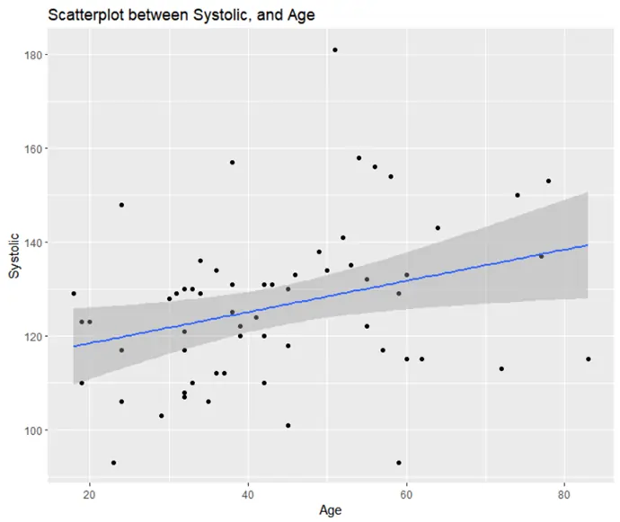
Figure 2: Scatterplot of Age and Systolic Blood Pressure
The scatterplot suggested a weak linear relationship between age and systolic blood pressure. We proceeded to conduct a linear regression with systolic blood pressure as the dependent variable and age as the predictor.
The null and alternative hypotheses for the regression were defined as follows:
- H0: βage = 0 (No significant relationship)
- H1: βage ≠ 0
The significance level was set at 5%. The results of the linear regression analysis are displayed in the table below.
| Coefficients | Estimate | Std. Error | t-value | P-value |
|---|---|---|---|---|
| Intercept | 111.78 | 6.22 | 19.97 | 0.001 |
| Age | 0.33 | 0.13 | 2.48 | 0.0162 |
Table 3: Linear Regression for Systolic Blood Pressure by Age
The linear regression model explained a statistically significant but weak proportion of variance (R2 = 0.10). The effect of age was statistically significant and positive (beta = 0.33, t(58) = 2.48, p = 0.016).
Conclusion
Based on the regression analysis, there was a weak, positive, and statistically significant relationship between age and systolic blood pressure.
Part 3: Exploring Correlations Between Time in Australia and Hypertension
Research Question: Do the data provide evidence to suggest that the length of time spent in Australia (Time) is correlated with whether participants have hypertension?
Analysis
To address this research question, we used a chi-squared test of independence. Initially, we created a stacked bar chart to visualize the proportions of hypertension for each time category.
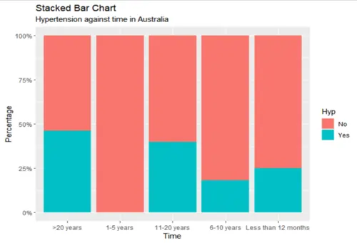
Figure 3: Stacked Bar Chart of Hypertension by Time
Based on the bar chart, there appeared to be some association between hypertension and time. The null and alternative hypotheses for the chi-squared test were defined as follows:
- H0: There is no association between time and hypertension
- H1: H0 is false
The significance level was set at 5%. The results of the chi-squared test are presented in the table below.
| Time | No | Yes |
|---|---|---|
| 20 years | 7 | 6 |
| 1-5 years | 14 | 0 |
| 11-20 years | 6 | 4 |
| 6-10 years | 9 | 2 |
| 12 months | 9 | 3 |
Table 4: Chi-squared Test of Independence for Time and Hypertension
The chi-squared test yielded a statistically insignificant result (χ2 = 9.242, p = 0.055). The test indicated that the strength of association between time and hypertension was not strong enough to be considered significant.
Conclusion
Our analysis concluded that there was no significant correlation between hypertension and the time participants spent in Australia.
Summary
This assignment demonstrates the application of statistical methods and R programming skills to analyze data related to well-being. It showcases the use of descriptive statistics, ANOVA, linear regression, and chi-squared tests to address pertinent research questions related to BMI, systolic blood pressure, age, and their relationships with other variables.
Related Samples
Embark on a journey through our sample section, where a plethora of statistical examples await. Immerse yourself in practical demonstrations spanning regression analysis, data visualization, and more. Uncover comprehensive case studies designed to bolster your comprehension and analytical skills. Let our curated samples serve as your guide in navigating the complexities of statistical methodology.
Data Analysis
R Programming
Data Analysis
Data Analysis
Data Analysis
Statistics
Data Analysis
tableau
R Programming
Data Analysis
Data Analysis
Data Analysis
Data Analysis
Data Analysis
Data Analysis
R Programming
Data Analysis
Data Analysis
Data Analysis
Data Analysis