How to Approach and Solve Supply Chain Optimization Assignments Using Linear Programming

Step 1: Understanding the Problem Statement

The first step in solving a supply chain optimization problem is to thoroughly analyze the given information, which typically includes:

• The number of manufacturing plants and their capacities.
• Distribution centers and their respective demand requirements.
• The transportation cost matrix from each plant to each distribution center.
• Possible expansion options for existing plants or establishment of new plants.

By carefully extracting these details, students can ensure they accurately define the constraints and objectives of the problem. Ignoring any key data point may result in suboptimal solutions that do not fully address the problem’s constraints and cost considerations.

A strong understanding of the given supply chain problem also enables students to identify redundant costs and bottlenecks. Often, inefficiencies in transportation routes or plant utilization can lead to increased expenses. Therefore, paying close attention to the problem statement helps in formulating an effective optimization model.

Step 2: Defining Decision Variables

Decision variables represent the quantities of goods transported between different locations. For instance:

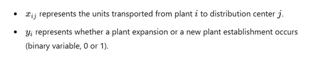
Clearly defining these decision variables is crucial because they form the foundation of the LP model. Incorrect definitions can lead to infeasible solutions, where either supply exceeds capacity or demand is not met. Furthermore, precise decision variables help in effectively communicating the model to stakeholders and facilitating computational implementation.

Step 3: Formulating the Objective Function

In most supply chain optimization problems, the objective is to minimize total transportation and facility costs:

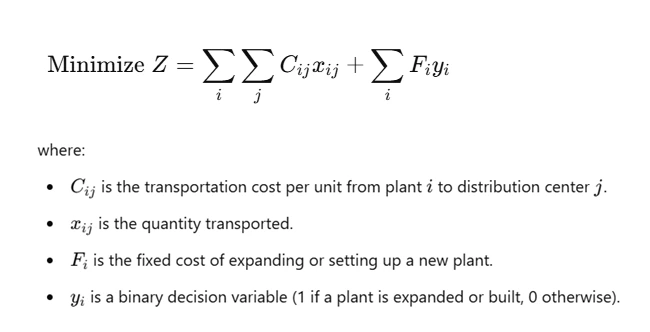
This function aims to strike a balance between fulfilling demand and minimizing costs. In real-world applications, additional considerations such as lead times, regulatory constraints, and carbon footprint reduction may also be incorporated into the objective function.

Step 4: Defining Constraints

The model must adhere to several key constraints:

1. Supply Constraints

Each manufacturing plant cannot supply more than its available capacity:

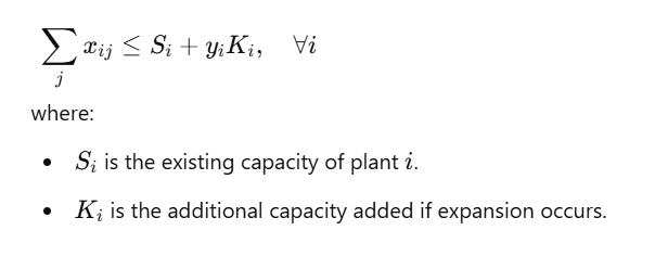
Supply constraints ensure that plants do not exceed their maximum output, which could otherwise lead to infeasible solutions. In industries with fluctuating production capabilities, supply constraints may also account for seasonal variations.

2. Demand Fulfillment Constraints

Each distribution center must receive the required demand:

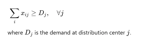
This constraint ensures customer satisfaction by meeting demand obligations. Failure to meet demand could result in lost sales and reputational damage. Some supply chain models also introduce penalty costs for unfulfilled demand.

3. Non-Negativity and Binary Constraints

Quantities shipped must be non-negative, and facility decisions must be binary:

Step 5: Implementing and Solving the Model

Once the LP model is formulated, it can be solved using tools like:

• Excel Solver
• AMPL
• Python (PuLP, Gurobi, or CPLEX)

By inputting the objective function and constraints into these tools, students can determine the optimal transportation plan and facility decisions. The choice of solver depends on the complexity of the problem and the available computational resources. Some advanced solvers also allow stochastic modeling, which incorporates uncertainty in demand and supply forecasts.

Step 6: Interpreting and Visualizing Results

After obtaining the solution, it is crucial to:

• Identify total transportation and expansion costs.
• Analyze whether demand is fully met.
• Visualize the optimal flow using network diagrams.
• Conduct sensitivity analysis on variables like demand changes.

Visualization techniques such as Sankey diagrams or heatmaps help in understanding the cost distribution and potential bottlenecks in the supply chain. Additionally, performing scenario analysis on fluctuating demand levels can provide deeper insights into the robustness of the optimization model.

Step 7: Evaluating Expansion and New Plant Options

Many assignments include options for increasing capacity. In such cases:

• Fixed charge problems are used to determine the best expansion choice.
• Sensitivity analysis helps evaluate different demand scenarios.

For example, if demand in Shanghai fluctuates between 20,000 and 90,000 units, rerunning the model under different conditions provides insights into the most resilient supply chain configuration. Sensitivity analysis aids in determining whether expanding an existing plant or establishing a new one is the optimal solution.

Conclusion

Solving supply chain optimization assignments requires a methodical approach, including problem analysis, LP model formulation, implementation, and result interpretation. By mastering these steps, students can effectively tackle similar assignments and gain proficiency in prescriptive analytics techniques for real-world decision-making.

A well-optimized supply chain ensures cost-effectiveness and efficient resource utilization. Understanding these concepts is essential for students aspiring to build careers in logistics, operations research, and business analytics. With continual advancements in data analytics and machine learning, future supply chain models will incorporate predictive analytics to make even more informed decisions based on real-time data. By developing a strong foundation in these optimization techniques, students will be well-equipped to handle complex logistics challenges in their professional careers. For those looking for assistance in tackling assignments related to these complex topics, Statistics Assignment Help can provide valuable support in understanding the mathematical models and statistical methods behind supply chain optimization. This resource can guide students in mastering key concepts like linear programming and data analysis, helping them succeed in their academic journey.